blog

Dijkstra's Algorithm

5th Dec 2020

While sitting in a café in 1956, Edsger Dijkstra considered the problem of finding the shortest path between two cities, namely Rotterdam and Groningen. In around 20 minutes, he designed what would be later coined Dijkstra's Algorithm to do exactly this. Three years later, he published a short paper titled A Note on Two Problems in Connexion with Graphs¹ which describes the workings of the algorithm.

Many decades later, this algorithm and its variants are used extensively in many domains such as travel navigation, packet routing and social networking. This blog post will explain how Dijkstra's algorithm works, based on the implementation in CLRS².

The Single-Source Shortest Paths Problem

Consider the case where we have a weighted, directed graph $G=(V, E)$ where $V$ is the set of vertices and $E$ is the set of edges. The goal of the single-source shortest paths problem is to find the shortest path from a single vertex $s$ to each node in the graph $v \in V$. Dijkstra's Algorithm is one solution to this problem.

Shortest Path Estimate and Predecessors

Throughout Dijkstra's Algorithm, two important attributes are maintained for each vertex in the graph. The first of these is the shortest path estimate, $d$. This represents the weight of the path from $s$ to a particular vertex $v$ which the algorithm considers to be the shortest at a particular point in time during the execution of the algorithm. This value will be continually updated throughout execution as shorter paths are discovered.

The next important attribute is $\pi$, which is used to represent a vertex's predecessor on the current shortest path. For example, if the current shortest path from $s$ to $v$ is $s\rightarrow a \rightarrow b \rightarrow c \rightarrow v$, then the predecessor of $v$ is $c$. Every time a better estimate is found for the shortest path to a particular node $v$, $v.d$ must be updated to indicate the weight of this path and $v.\pi$ must be updated to indicate the predecessor of $v$ on the current shortest path.

Initialization

At the beginning of the algorithm, only one shortest path in the graph is known. This is the path from the source vertex $s$ to itself. Therefore, the $d$ value for this vertex can be set to 0, as the path weight to get from $s$ to itself is 0, and the predecessor of this vertex can be set to $NIL$.

For every other vertex in graph, no shortest path is known, nor does the algorithm have any estimate for what these paths might be. Therefore, for each of these vertices, $d$ is set to $\infty$ and $\pi$ is set to $NIL$. Throughout execution, the algorithm will continually update these values whenever a better estimate for each shortest path is found. The pseudocode for the initialization process is shown below:²

# INITIALIZE-SINGLE-SOURCE(G, s)

for each vertex v ∈ G.V
    v.d = ∞
    v.π = NIL
s.d = 0

Processed and Unprocessed Vertices

After initialization, the main loop of Dijkstra's Algorithm selects a vertex at a time and completes a process called relaxation, as described in the following section. However, the order in which the nodes are processed must be determined. This is done by maintaining a min priority queue, $Q$, which is keyed by the vertices' $d$ values. For each iteration of the main loop, the vertex with the lowest priority (i.e. the lowest $d$ value) is pulled from the queue. This vertex $u$ is then moved from $Q$ into the set $S$, before relaxing the edges leaving $u$. Therefore, $S$ contains all of the vertices for which their shortest path estimate is the actual shortest path. I will not prove this here, but please check CLRS for the full proof.

Relaxation

The first step of the main loop of Dijkstra's Algorithm is to pull the vertex $u$ with the lowest $d$ value from $Q$, and add it to the set $S$. Following this, the edges leaving $u$ must be relaxed. The process of relaxing an edge $(u,v)$ determines whether the shortest path estimate to $v$ can be improved by going through $u$. If it can, then vertex $v$'s $d$ value is updated to reflect the weight of this new path and its $\pi$ value is set to $u$. The pseudocode for this is shown below:²

# RELAX(u, v, w)

if v.d > u.d + w(u, v)
    v.d = u.d + w(u, v)
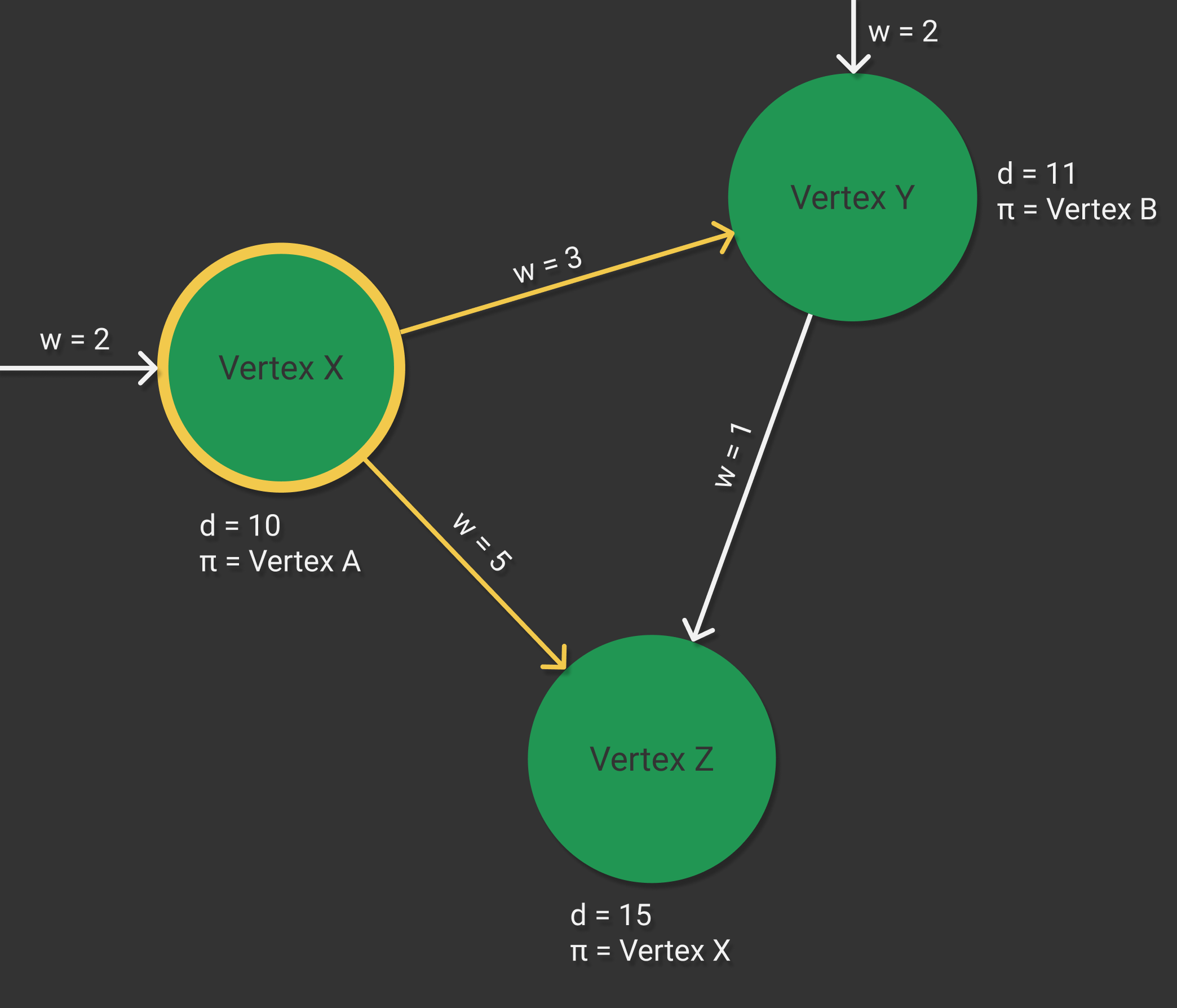
    v.π = u

Consider the case where we have a section of a graph with vertices $X$, $Y$ and $Z$, as shown below. The graph is currently in a state where the edges leaving $X$ have already been relaxed, as indicated in yellow. When relaxing edge $(X, Y)$, the algorithm first checked if the current shortest path weight for $X$ plus the weight of the edge $(X, Y)$ was less than the shortest path estimate for $Y$, as described in the pseudocode shown above. In this case, it was not, and so the shortest path estimate and predecessor for $Y$ were not updated.

Prior to this relaxation, the shortest path estimate for $Z$ was $\infty$. When the edge $(X, Z)$ was relaxed, the algorithm calculated the shortest path estimate of $X$ plus the weight of the edge $(X, Z)$, which resulted in $10 + 5 = 15$. As $15<\infty$, the shortest path estimate for $Z$ was updated to $15$ and the predecessor value was updated to $X$.

Dijkstra's Algorithm

Now that we have described all of the concepts individually, I will now explain Dijkstra's Algorithm in full. First, the algorithm is initialized by setting the shortest path estimate for the source node to $0$; setting the shortest path estimates for the other nodes to $\infty$; and setting the predecessor values for each node to $NIL$. The algorithm then creates an empty set $S$ to store the vertices for which it is known that their shortest path estimate is the shortest path. A min-priority queue, $Q$, is then created by taking the set of vertices $V$ and keying them by their $d$ values.

From here, the main loop can then start. For each iteration of this loop, the vertex $u$ with the minimum shortest path estimate is extracted from the priority queue. This vertex is then added to the set $S$, which indicates that the shortest path estimate for this node is the shortest path. The algorithm then iterates over the vertices that share an edge with $u$, and relaxes these edges. This process involves updating the shortest path estimates and predecessors for these vertices if a shorter path can be achieved by going through $u$. Once all edges have been relaxed, the next iteration of the while loop continues, extracting the vertex with the minimum shortest path estimate from the priority queue. This process continues until $Q$ is empty. The pseudocode for this algorithm is shown below:²

# DIJKSTRA(G, w, s)

INITIALIZE-SINGLE-SOURCE(G, s)
S = Ø
Q = G.V
while Q ≠ Ø
    u = EXTRACT-MIN(Q)
    S = S ∪ {u}
    for each vertex v ∈ G.Adj[u]
        RELAX(u, v, w)

As mentioned at the beginning, a solution to the single-source shortest paths problem should be able to find the shortest path from $s$ to any vertex $v$ in a graph. After the execution of Dijkstra's Algorithm, the set $S$ will contain all of the vertices in the graph, where all of the shortest path estimates are the shortest paths, and all of the $\pi$ values point to the predecessor values on the shortest path to each vertex. To find the shortest path from $s$ to a particular vertex $v$, we can simply find $v$ in the set $S$ and traverse back through the predecessor vertices indicated by the $\pi$ values until we reach $s$. Therefore, Dijkstra's Algorithm is a complete solution to the single-source shortest paths problem.

For further reading on this topic, please check out the full proof for this algorithm in the CLRS textbook, and Dijkstra's original 1959 paper - both of which are included in the bibliography below.

Bibliography

1. E. W. Dijkstra, A Note on Two Problems in Connexion with Graphs. 1959.
2. T. Cormen, C. Leiserson, R. Rivest and C. Stein, Introduction to Algorithms.