blog

Dynamic Programming: Top-Down vs Bottom-Up

31st Jan 2021

Dynamic Programming is a method used to solve problems by breaking the main problem into subproblems, storing and reusing the results, and combining the solutions. This may sound similar to the heavily-used algorithmic technique Divide and Conquer, however there is a key distinction. Dynamic Programming algorithms store and reuse the results of each subproblem, meaning that each distinct subproblem is solved only once.¹

One of the most fundamental applications of Dynamic Programming is to calculate the $n^{th}$ number in the Fibonacci sequence. The beginning of the sequence is shown below:

In order to calculate the Fibonacci number at any index $n$, we can use the following equation, which says that the Fibonacci number at any index $n$ is equal to the sum of the two previous numbers in the sequence.

The sequence starts with $fib(0) = 0$ and $fib(1)=1$. Knowing these two values, succeeding Fibonacci numbers can be calculated indefinitely. The value of $fib(2)$ can be calculated by summing $fib(1)+fib(0)=1$; the value of $fib(3)$ can be calculated by summing $fib(2)+fib(1)=2$; and so on. Whenever the Fibonacci number at index $n$ is calculated, we can use this result along with the value of $fib(n-1)$ to compute the value of $fib(n + 1)$.

Requirements for Dynamic Programming

In order for Dynamic Programming to be applied to a problem, the problem itself must have two properties:

• Optimal Substructure
• Overlapping Subproblems

If an optimal solution to a problem can be constructed from optimal solutions of its subproblems, then the problem is said to have optimal substructure. For the problem of calculating Fibonacci numbers, this property holds true. For example, the solution to $fib(6)$ is calculated by finding the sum of the two subproblems: $fib(5)$ and $fib(4)$. Similarly, the solution to $fib(5)$ is the sum of $fib(4)$ and $fib(3)$; the solution to $fib(4)$ is the sum of $fib(3)$ and $fib(2)$; and so on. The diagram below shows this visually.

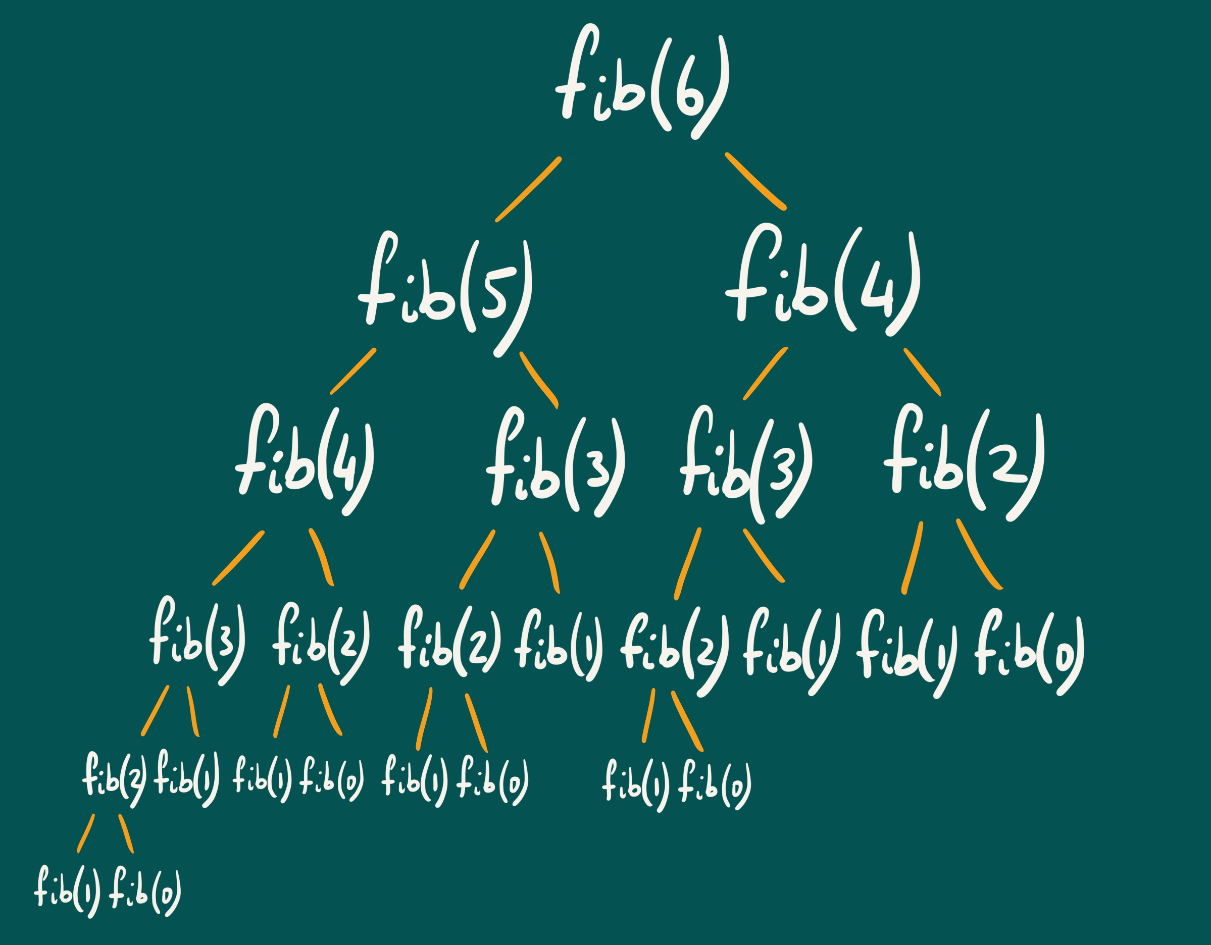
The next requirement is Overlapping Subproblems. This property states that the solution to a problem must contain subproblems that are solved multiple times. Looking at the diagram above, we can see that $fib(2)$ is calculated $5$ times; $fib(3)$ is calculated $3$ times; $fib(4)$ is calculated twice; etc. Dynamic Programming aims to optimise this by removing the need to calculate the results of each subproblem more than once.

Terminology

If a problem has both of these properties, then there are two possible Dynamic Programming implementations than can be used:

• Recursive Top-Down with Memoization
• Iterative Bottom-Up

In some cases, the term Dynamic Programming is only used to refer to the Iterative Bottom-Up approach, and the term Memoization is used to refer to the Recursive Top-Down with Memoization approach². However, in this blog post I will use the terminology used in the CLRS¹ textbook, which uses Dynamic Programming to refer to both approaches.

Recursive Top-Down Solution

Before moving on to the Dynamic Programming solutions, it is useful to show how a simple recursive algorithm can be used to solve the Fibonacci problem. The recursive solution simply calculates $fib(n)$ by first checking if $n$ is equal to $0$ or $1$ — in which case the solution is $0$ or $1$ respectively — and if not, returning the result of $fib(n-1) + fib(n-2)$. These recursive calls then call the same method again with a lower value of $n$. This only stops when the algorithm already knows the solution for that particular value of $n$, which only occurs for $n=0$ or $n=1$ in this case. As shown in the previous diagram, this solution does a lot more work than necessary, as many of the subproblems are solved multiple times.

FIB(n)
1   if n == 0 or n == 1 then
2      return n
3   return FIB(n-1) + FIB(n-2)

Recursive Top-Down with Memoization

Another way of solving the problem of calculating Fibonacci numbers is to use the Recursive Top-Down with Memoization implementation of Dynamic Programming. This is very similar to the recursive solution explained previously, with one key difference: memoization. Memoization is the process of saving the results of calculations so that they can be used later in the execution of the algorithm when the same input occurs again. As a result of this, the recursion tree now drastically reduces in size, as shown below:

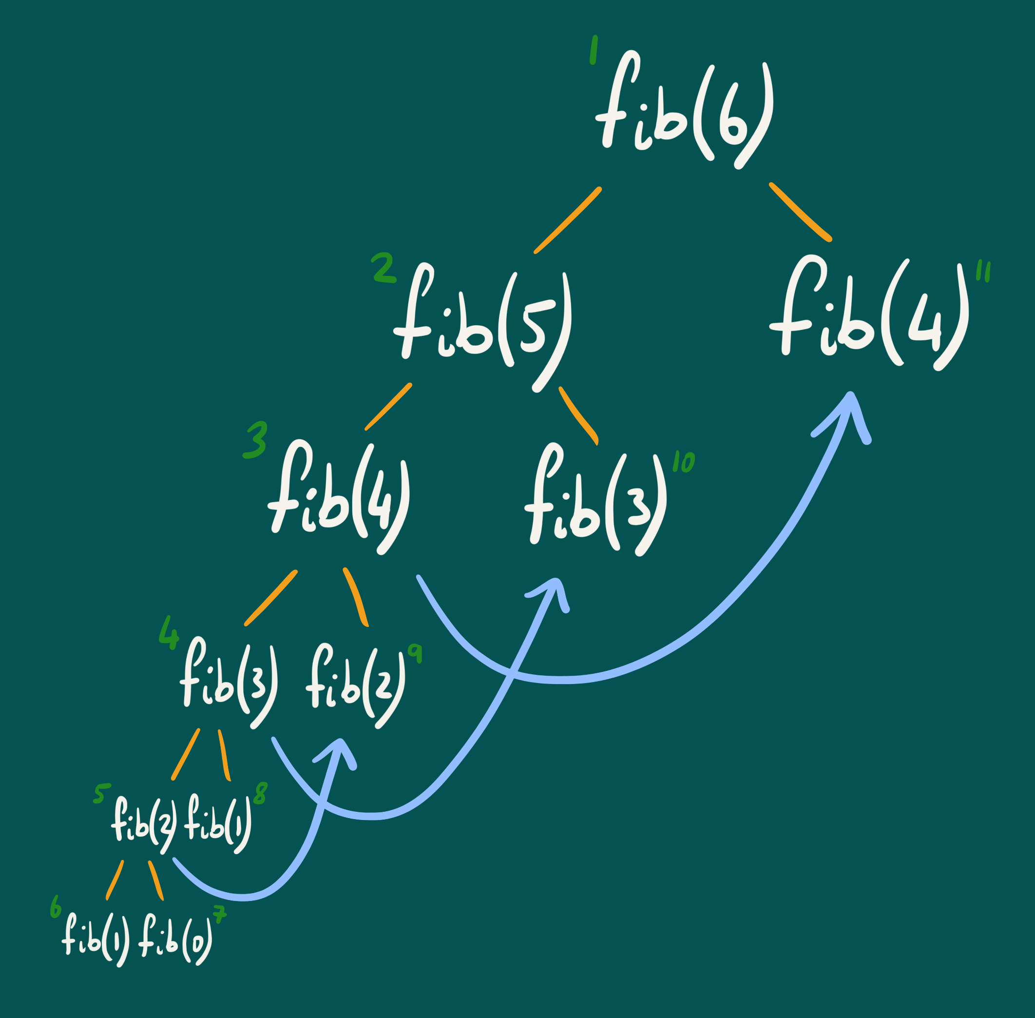
The numbers shown in green indicate the order of execution. Initially, when the algorithm tries to calculate $fib(6)$, it looks for the first subproblem that it needs to find a solution to, which in this case is $fib(5)$. Now, it will move on to find the solution to the first subproblem needed to calculate $fib(5)$, which in this case is $fib(4)$. Similarly, it will continue to find a solution to the first subproblem needed to calculate $fib(4)$, which in this case is $fib(3)$. This continues until one of the base cases, $fib(0)$ or $fib(1)$, is reached. At this point, the algorithm can start moving back up the tree and solving the remaining subproblems. As shown on the diagram, the remaining subproblems have already been solved, so the solutions can simply be reused (indicated by the blue lines on the diagram), removing huge parts of the recursion tree. The pseudocode for this solution is shown below:

FIB-INIT(n)
1   memo = array of size n + 1 init 0
2   return FIB(n, memo)

FIB(n, memo)
1   if (n == 0 or n == 1) then
2      return n
3   if memo[n] != 0 then
4      return memo[n]
5   result = FIB(n-1, memo) + FIB(n-2, memo)
6   memo[n] = result
7   return result

Iterative Bottom-Up

The second implementation of Dynamic Programming that can be used to solve the Fibonacci problem is the Iterative Bottom-Up approach. In short, this algorithm starts by calculating the solution to the simplest case, before iteratively moving towards the desired value of $n$.

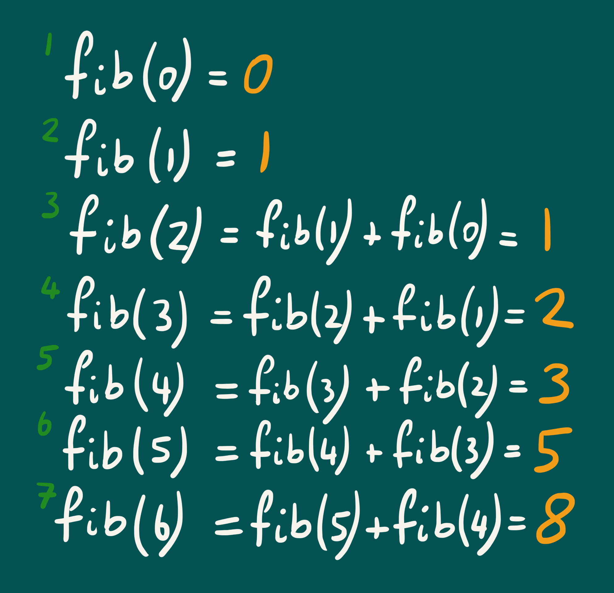
For example, to calculate $fib(6)$, the algorithm will start with $fib(0)$ and iteratively calculate solutions for increasing values of $n$, only stopping when $n = 6$. Due to the fact that $n$ is increasing, whenever the algorithm is trying to calculate $fib(n)$ at any point, the solutions to $fib(n-1)$ and $fib(n-2)$ will already be known. This is shown in the diagram above, where the values in green indicate the order of execution. The pseudocode for this solution is shown below:

FIB(n)
1   if (n == 0 or n == 1) then
2      return n
3   minusTwo = 0
4   minusOne = 1
5   fib = 0
6   for i = 2 to n-1
7      fib = minusTwo + minusOne
8      minusTwo = minusOne
9      minusOne = fib
10  return fib

As shown, Dynamic Programming is an extremely powerful technique that can be used to achieve huge optimisations. The Fibonacci problem explained in this blog post is a simple and intuitive example used to illustrate the effectiveness of Dynamic Programming, however there are a plethora of other use cases. For further reading on this topic, please check out the brilliant Dynamic Programming examples in the CLRS textbook.¹

Bibliography

1. T. Cormen, C. Leiserson, R. Rivest and C. Stein, Introduction to Algorithms.
2. G. Laakmann Mcdowell, Cracking the Coding Interview.